Important additions to Statgraphics 18 are 4 procedures for equivalence and noninferiority testing: comparison of 2 independent means, comparison of 2 paired means, comparison of 2 means using a 2x2 crossover study, and comparison of a mean to a target value. In each case, the tests are designed to demonstrate that a test formulation or treatment gives equivalent or better results than a reference treatment. This is in marked contrast to most hypothesis tests that are designed to demonstrate differences rather than similarities.

Searching the Internet, I have found many interesting examples of this type of testing: comparison of a generic drug to a brand-name drug, comparison of genetically modified feedstuffs for livestock to standard feedstocks, assessment of health disparities in vaccination coverage among different groups of people,  comparison of implicit and explicit measures of self-esteem, comparison of measurement systems, evaluation of changes in manufacturing equipment, comparison of different instruments in sensory and consumer research, and many more.

Bioequivalence

Many applications have to do with demonstrating "bioequivalence", which is defined by the FDA as: "the absence of a significant difference in the rate and extent to which the active ingredient or active moiety in pharmaceutical equivalents or pharmaceutical alternatives becomes available at the site of drug action when administered at the same molar dose under similar conditions in an appropriately designed study." Or more simply, the 2 drugs have equivalent effects. Of course, equivalent doesn't mean exactly the same. Often it means that a 95% confidence interval for their relative difference lies completely within the interval from 80% to 125%.

2x2 Crossover Studies

A very common experimental design for demonstrating equivalence or noninferiority is a 2x2 crossover study. In such a study, 2 treatments (A and B) are administered to a group of subjects. Half the subjects get treatment A followed by treatment B, while the other half get treatment B followed by treatment A. Administration of the treatments is assumed to be separated by enough time that the effect of the first treatment does not carryover and affect the outcome of the second treatment, an assumption which must be tested as part of the analysis. You'll find a special procedure in Statgraphics 18 for analyzing these types of studies.

As an example consider the following data from a study published in Chow and Liu (2009):

24 patients were given both a reference formulation and a test formulation. 12 patients were randomly selected and assigned to the sequence RT in which the reference formulation was administered first, while the other 12 patients were assigned to sequence TR and received the test formulation first. By applying both treatments to the same subjects, between-subject differences can be blocked out of the analysis allowing for more powerful tests.

The figure below plots the measurements for each of the 24 patients.

The location along the X-axis is the measurement made in period 1 (corresponding to the first formulation administered), while the location along the Y-axis is the measurement made in period 2. The color of the points indicates which sequence each patient was assigned to.

Constructing the Hypothesis Test

Suppose for a moment that patients when administered the reference treatment have a mean outcome equal to μ_R and that patients when administered the test treatment have a mean outcome equal to μ_T. Suppose also that our goal is to demonstrate that the ratio of the test treatment mean to the reference treatment mean is between 80% and 125%. As our null hypothesis, we would suppose that the ratio of the means is either less than 80% or greater than 125%:

H₀: μ_T/μ_R < 0.80  or  μ_T/μ_R > 1.25

Our alternative hypothesis (the one we wish to demonstrate) is that the ratio is within the indicated range:

H_A: 0.8 ≤ μ_T/μ_R ≤ 1.25

Note that this is basically the reverse of a standard hypothesis test in which the null hypothesis rather than the alternative hypothesis would indicate no difference between the 2 means.

Statistical Model

The best way to understand the statistical model for this data is to examine the expected values for patients in each sequence during each time period as shown below:

where S is a sequence effect, P is a period effect, and λ_R and λ_T are carryover effects of the reference and test formulations, respectively. A carryover effect is the effect of the treatment from the previous time period on the response at the current time period. In the above table, the effects are shown as additive. Alternatively, it is sometimes assumed that the effects are multiplicative, in which case there are 2 choices: (1) an additive model may be used to analyze logarithms rather than the original measurements, or (2) Fieller’s theorem may be applied using the method outlined by Locke (1984).

If the means of the two formulations are estimated by averaging the results of all patients when given that formulation, the difference between the treatment means is not aliased with either the sequence or period effects if the design is balanced (same number of patients in each sequence). However, the difference between the means is aliased with the crossover effects unless the crossover effects of the test and reference formulations are equal. Consequently, when performing such a study, an attempt must be made to separate the administration of the 2 formulations by enough time such that the effect of the formulation administered first has dissipated (a washout period).

TOST (Two One-Sided Tests)

The most common way of performing equivalence tests uses a procedure called TOST (two one-sided tests). 2 separate hypothesis tests are performed using hypotheses such as:

Test 1
H₀: μ_T/μ_R < 0.80 
H_A: μ_T/μ_R ≥ 0.80

Test 2
H₀: μ_T/μ_R > 1.25
H_A: μ_T/μ_R ≤ 1.25

If both null hypotheses are rejected at the α% significance level, then equivalence between the means will have been demonstrated at that significance level.

Data Analysis

Statgraphics 18 contains a new procedure for analyzing the results of 2x2 crossover studies. Is it accessed by selecting Compare on the main menu and then choosing Equivalence and Noninferiority Tests – 2x2 Crossover Study. The names of the columns are entered on the data input dialog box as shown below:

The Analysis Options dialog box is used to specify the hypotheses to be tested:

The settings shown above indicate that a two-sided equivalence test is desired, based on the ratio of the means. Equivalence may be asserted if the ratio is between 0.8 and 1.25 using an α-level of 5%. The analysis will be based on an additive model for the logarithms of the recorded data.

Several tables are produced by the procedure, the first of which shows the results of fitting the statistical model:

t-tests are performed to determine whether or not there are significant carryover, treatment and period effects. A significant carryover effect would indicate that the carryover effects of the test and reference formulations were significantly different, implying that the comparison of treatment means would be biased. A small P-value for the carryover effect would thus throw doubt on the entire equivalence analysis. A significant period effect would indicate that something happened between the first and second periods to cause all of the results to shift. Provided the design is balanced, this would not affect the comparison of the test and reference means but would indicate some unexpected change from one period to the next.

It is also useful to plot the estimated means of the test and reference formulations during the 2 periods:

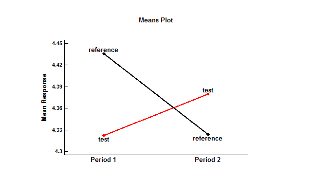
When applied first, the mean of the test formulation was slightly lower than the mean of the reference formulation. When applied second, the test mean was slightly higher. The results of a standard t-test of the difference between the means, shown in the previous table, did not reject the hypothesis that the means were identical. However, such a test does not demonstrate equivalence.

Equivalence Test

The second part of the Statgraphics 18 Analysis Summary shows the results of the TOST procedure:

The top section shows that the difference between the means of the logarithms for the test and reference formulations is approximately -0.0287, with a 95% confidence interval extending from -0.1243 to 0.0670. The estimated ratio of the means is approximately 0.972, with a 95% confidence interval extending from 0.883 to 1.609. Two t tests were performed to test the hypotheses shown earlier. Test #1 shows that the ratio is significantly greater than 0.8 (lower P-Value well below 0.05). Test #2 shows that the ratio is significantly less than 1.25 (upper P-Value well below 0.05). Since the larger of the 2 P-values is less than 0.05, equivalence between the test and reference means has been demonstrated at the 5% significance level.

Equivalence Plot

It is also helpful to plot the results. The plot below shows a 95% confidence interval for the ratio of the test mean to the reference mean:

Note that the entire confidence interval falls between the lower equivalence limit (LEL) and the upper equivalence limit (UEL). This will be the case whenever the TOST procedure concludes that the means are equivalent.

Note on Confidence Limits

When equivalence testing was first developed, it was common practice to display a 90% confidence interval for the difference between the means using the formula

where

,

s_p is the pooled standard deviation of the within-subject differences in the 2 sequences, and ν is the degrees of freedom associated with s_p. In recent years, it has become standard practice to calculate a 95% confidence interval instead using the formula

Either approach has the property that whenever the TOST procedure indicates that the means are equivalent, the calculated interval will be completely within the limits. Statgraphics 18 applies the second formula by default, although an option on the Analysis Options dialog box allows the analyst to use the first formula if desired.

One-Sided Noninferiority Tests

In some cases, the goal of the analysis is not to show that a test and reference mean are “equivalent”, but only to show that the test formulation is at least as good as the reference formulation. In such cases, only one of the 2 one-sided tests described above in the TOST section needs to be performed. For example, if we wish to demonstrate that the test mean is at least 80% as large as the reference mean, we would specify hypotheses such as

Test 1
H₀: μ_T/μ_R < 0.80 
H_A: μ_T/μ_R ≥ 0.80

Rejection of the null hypothesis would then imply that the test mean is “not inferior” to the reference mean. The two-sided 95% confidence interval is replaced by a one-sided 95% confidence bound as shown below:

Further Information

There's an excellent discussion of these topics in the Journal of General Internal Medicine which you can read online titled Understanding Equivalence and Noninferiority Testing. A thorough discussion of crossover trials is given by Li (2014). I've also recorded 4 videos on the topic which you will find listed on our Instructional Videos page.

References

Berger, R.L. and Hsu, J.C. (1995). “Bioequivalence trials, intersection-union tests, and equivalence confidence sets.” Institute of Statistics Mimeo Series Number 2279.

Chow, S.C. and J.P. Liu. (2009). Design and Analysis of Bioavailability and Bioequivalence Studies. 3rd ed. Boca Raton, FL: CRC Press.

Chow, S.-H. and Shao, J. (2002). Statistics in Drug Research: Methodologies and Recent Developments. New York: Marcel-Dekker.

Hsu, J.C., Hwang, J.T.G., Liu, H.-K., and Ruberg, S.J. (1994). “Confidence intervals associated with tests for bioequivalence.” Biometrika 81: 103-114.

Jones, B. and Pang, H.  (2014) Design and Analysis of Crossover Trials. 3rd ed. Boca Raton, FL: CRC Press.

Li, C.S. (2014) Design and Analysis of Crossover Trials. www.ucdmc.ucdavis.edu/mindinstitute/centers/iddrc/pdf/bbrd_oct_2014.pdf

Locke, C.S. (1984). “An exact confidence interval for untransformed data for the ratio of two formulation means.” J Pharmacokinet Biopharm 12: 649-655.

Niazi, S.K. (2014). Handbook of Bioequivalence Testing. 2^nd ed. Drugs and the Pharmaceutical Sciences. Boca Raton, FL: CRC Press.

Patterson, S.D. and Jones, B. (2016). Bioequivalence and Statistics in Clinical Pharmacology. 2nd ed. Boca Raton, FL: CRC Press.

Ng, T. (2015) Noninferiority Testing in Clinical Trials: Issue and Chanllenges. Boca Raton, FL: CRC Press.

Pardo, S. (2013) Equivalence and Noninferiority Tests for Quality, Manufacturing and Test Engineers. Boca Raton, FL: CRC Press.

Rothmann, M.D., Wiens, B.L., and Chan, I.S.F. (2011) Design and Analysis of Noninferiority Trials. Boca Raton, FL: CRC Press.

Schuirmann, D.J. (1987). “A comparison of the one-sided tests procedure and the power approach for assessing the equivalence of average bioavailability.” J Pharmacokinet Biopharm 15: 657-680.

U.S. Department of Health and Human Services, Agency for Healthcare Research and Quality (2013) Assessing Equivalence and Noninferiority.

Wellek, S. (2010) Testing Statistical Hypotheses of Equivalence and Noninferiority, 2^nd ed. Boca Raton, FL: CRC Press.

Yu, L.X. and Li, B.V. eds. (2014). FDA Bioequivalence Standard (AAPS Advances in Pharmaceutical Sciences Series). Springer: AAPS Press.